CNN Implementation
CNN Implementation
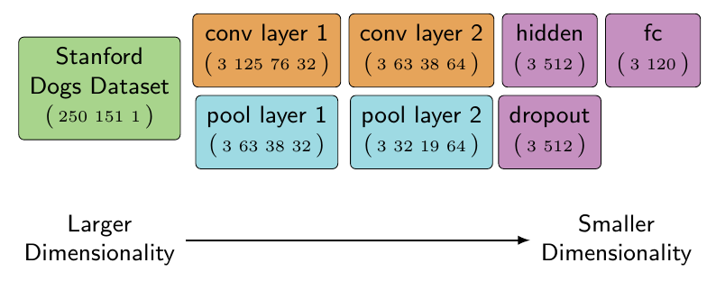
Object recognition and categorization using TensorFlow required a basic understanding of convolutions (for CNNs), common layers (non-linearity, pooling, fc), image loading, image manipulation and colorspaces. With these areas covered, it’s possible to build a CNN model for image recognition and classification using TensorFlow. In this case, the model is a dataset provided by Stanford which includes pictures of dogs and their corresponding breed. The network needs to train on these pictures then be judged on how well it can guess a dog’s breed based on a picture.
The network architecture follows a simplified version of Alex Krizhevsky’s AlexNet without all of AlexNet’s layers. This architecture was described earlier in the chapter as the network which won ILSVRC'12 top challenge. The network uses layers and techniques familiar to this chapter which are similar to the TensorFlow provided tutorial on CNNs.
Stanford Dogs Dataset
The dataset used for training this model can be found on Stanford’s computer vision site http://vision.stanford.edu/aditya86/ImageNetDogs/. Training the model requires downloading relevant data. After downloading the Zip archive of all the images, extract the archive into a new directory called imagenet-dogs in the same directory as the code building the model.
The Zip archive provided by Stanford includes pictures of dogs organized into 120 different breeds. The goal of this model is to train on 80% of the dog breed images and then test using the remaining 20%. If this were a production model, part of the raw data would be reserved for cross-validation of the results. Cross-validation is a useful step to validate the accuracy of a model but this model is designed to illustrate the process and not for competition.
The organization of the archive follows ImageNet’s practices. Each dog breed is a directory name similar to n02085620-Chihuahua where the second half of the directory name is the dog’s breed in English (Chihuahua). Within each directory there is a variable amount of images related to that breed. Each image is in JPEG format (RGB) and of varying sizes. The different sized images is a challenge because TensorFlow is expecting tensors of the same dimensionality.
Convert Images to TFRecords
The raw images organized in a directory doesn’t work well for training because the images are not of the same size and their dog breed isn’t included in the file. Converting the images into TFRecord files in advance of training will help keep training fast and simplify matching the label of the image. Another benefit is that the training and testing related images can be separated in advance. Separated training and testing datasets allows continual testing of a model while training is occurring using checkpoint files.
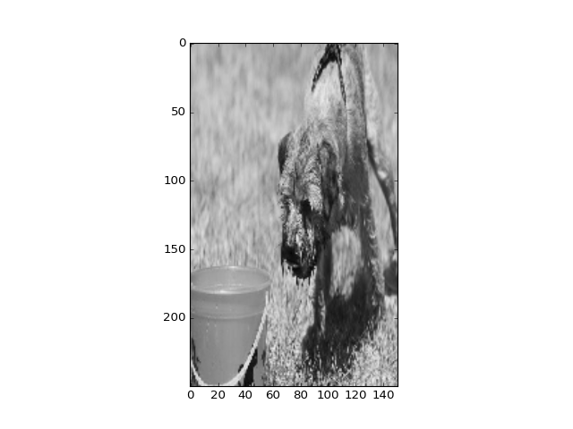
Converting the images will require changing their colorspace into grayscale, resizing the images to be of uniform size and attaching the label to each image. This conversion should only happen once before training commences and likely will take a long time.
# setup-only-ignore
import tensorflow as tf

sess = tf.InteractiveSession()
import glob

image_filenames = glob.glob("./imagenet-dogs/n02*/*.jpg")

image_filenames[0:2]
['./imagenet-dogs/n02085620-Chihuahua/n02085620_10074.jpg',
 './imagenet-dogs/n02085620-Chihuahua/n02085620_10131.jpg']
An example of how the archive is organized. The glob module allows directory listing which shows the structure of the files which exist in the dataset. The eight digit number is tied to the WordNet ID of each category used in ImageNet. ImageNet has a browser for image details which accepts the WordNet ID, for example the Chihuahua example can be accessed via http://www.image-net.org/synset?wnid=n02085620.
from itertools import groupby
from collections import defaultdict

training_dataset = defaultdict(list)
testing_dataset = defaultdict(list)

# Split up the filename into its breed and corresponding filename. The breed is found by taking the directory name
image_filename_with_breed = map(lambda filename: (filename.split("/")[2], filename), image_filenames)

# Group each image by the breed which is the 0th element in the tuple returned above
for dog_breed, breed_images in groupby(image_filename_with_breed, lambda x: x[0]):
    # Enumerate each breed's image and send ~20% of the images to a testing set
    for i, breed_image in enumerate(breed_images):
        if i % 5 == 0:
            testing_dataset[dog_breed].append(breed_image[1])
        else:
            training_dataset[dog_breed].append(breed_image[1])

    # Check that each breed includes at least 18% of the images for testing
    breed_training_count = len(training_dataset[dog_breed])
    breed_testing_count = len(testing_dataset[dog_breed])

    assert round(breed_testing_count / (breed_training_count + breed_testing_count), 2) > 0.18, "Not enough testing images."
This example code organized the directory and images (’./imagenet-dogs/n02085620-Chihuahua/n02085620_10131.jpg’) into two dictionaries related to each breed including all the images for that breed. Now each dictionary would include Chihuahua images in the following format:
training_dataset["n02085620-Chihuahua"] = ["n02085620_10131.jpg", ...]
Organizing the breeds into these dictionaries simplifies the process of selecting each type of image and categorizing it. During preprocessing, all the image breeds can be iterated over and their images opened based on the filenames in the list.
def write_records_file(dataset, record_location):
    """
    Fill a TFRecords file with the images found in `dataset` and include their category.

    Parameters
    ----------
    dataset : dict(list)
      Dictionary with each key being a label for the list of image filenames of its value.
    record_location : str
      Location to store the TFRecord output.
    """
    writer = None

    # Enumerating the dataset because the current index is used to breakup the files if they get over 100
    # images to avoid a slowdown in writing.
    current_index = 0
    for breed, images_filenames in dataset.items():
        for image_filename in images_filenames:
            if current_index % 100 == 0:
                if writer:
                    writer.close()

                record_filename = "{record_location}-{current_index}.tfrecords".format(
                    record_location=record_location,
                    current_index=current_index)

                writer = tf.python_io.TFRecordWriter(record_filename)
            current_index += 1

            image_file = tf.read_file(image_filename)

            # In ImageNet dogs, there are a few images which TensorFlow doesn't recognize as JPEGs. This
            # try/catch will ignore those images.
            try:
                image = tf.image.decode_jpeg(image_file)
            except:
                print(image_filename)
                continue

            # Converting to grayscale saves processing and memory but isn't required.
            grayscale_image = tf.image.rgb_to_grayscale(image)
            resized_image = tf.image.resize_images(grayscale_image, 250, 151)

            # tf.cast is used here because the resized images are floats but haven't been converted into
            # image floats where an RGB value is between [0,1).
            image_bytes = sess.run(tf.cast(resized_image, tf.uint8)).tobytes()

            # Instead of using the label as a string, it'd be more efficient to turn it into either an
            # integer index or a one-hot encoded rank one tensor.
            # https://en.wikipedia.org/wiki/One-hot
            image_label = breed.encode("utf-8")

            example = tf.train.Example(features=tf.train.Features(feature={
                'label': tf.train.Feature(bytes_list=tf.train.BytesList(value=[image_label])),
                'image': tf.train.Feature(bytes_list=tf.train.BytesList(value=[image_bytes]))
            }))

            writer.write(example.SerializeToString())
    writer.close()

write_records_file(testing_dataset, "./output/testing-images/testing-image")
write_records_file(training_dataset, "./output/training-images/training-image")
The example code is opening each image, converting it to grayscale, resizing it and then adding it to a TFRecord file. The logic isn’t different from earlier examples except that the operation tf.image.resize_images is used. The resizing operation will scale every image to be the same size even if it distorts the image. For example, if an image in portrait orientation and an image in landscape orientation were both resized with this code then the output of the landscape image would become distorted. These distortions are caused because tf.image.resize_images doesn’t take into account aspect ratio (the ratio of height to width) of an image. To properly resize a set of images, cropping or padding is a preferred method because it ignores the aspect ratio stopping distortions.
Load Images
Once the testing and training dataset have been transformed to TFRecord format, they can be read as TFRecords instead of as JPEG images. The goal is to load the images a few at a time with their corresponding labels.
filename_queue = tf.train.string_input_producer(
    tf.train.match_filenames_once("./output/training-images/*.tfrecords"))
reader = tf.TFRecordReader()
_, serialized = reader.read(filename_queue)

features = tf.parse_single_example(
    serialized,
    features={
        'label': tf.FixedLenFeature([], tf.string),
        'image': tf.FixedLenFeature([], tf.string),
    })

record_image = tf.decode_raw(features['image'], tf.uint8)

# Changing the image into this shape helps train and visualize the output by converting it to
# be organized like an image.
image = tf.reshape(record_image, [250, 151, 1])

label = tf.cast(features['label'], tf.string)

min_after_dequeue = 10
batch_size = 3
capacity = min_after_dequeue + 3 * batch_size
image_batch, label_batch = tf.train.shuffle_batch(
    [image, label], batch_size=batch_size, capacity=capacity, min_after_dequeue=min_after_dequeue)
This example code loads training images by matching all the TFRecord files found in the training directory. Each TFRecord includes multiple images but the tf.parse_single_example will take a single Example out of the file. The batching operation discussed earlier is used to train multiple images simultaneously. Batching multiple images is useful because these operations are designed to work with multiple images the same as with a single image. The primary requirement is that the system have enough memory to work with them all.
With the images available in memory, the next step is to create the model used for training and testing.
Model
The model used is similar to the mnist convolution example which is often used in tutorials describing convolutional neural networks in TensorFlow. The architecture of this model is simple yet it performs well for illustrating different techniques used in image classification and recognition. An advanced model may borrow more from Alex Krizhevsky’s AlexNet design which includes more convolution layers.
# Converting the images to a float of [0,1) to match the expected input to convolution2d
float_image_batch = tf.image.convert_image_dtype(image_batch, tf.float32)

conv2d_layer_one = tf.contrib.layers.convolution2d(
    float_image_batch,
    num_output_channels=32,     # The number of filters to generate
    kernel_size=(5,5),          # It's only the filter height and width.
    activation_fn=tf.nn.relu,
    weight_init=tf.random_normal,
    stride=(2, 2),
    trainable=True)
pool_layer_one = tf.nn.max_pool(conv2d_layer_one,
    ksize=[1, 2, 2, 1],
    strides=[1, 2, 2, 1],
    padding='SAME')

# Note, the first and last dimension of the convolution output hasn't changed but the
# middle two dimensions have.
conv2d_layer_one.get_shape(), pool_layer_one.get_shape()
(TensorShape([Dimension(3), Dimension(125), Dimension(76), Dimension(32)]),
 TensorShape([Dimension(3), Dimension(63), Dimension(38), Dimension(32)]))
The first layer in the model is created using the shortcut tf.contrib.layers.convolution2d. It’s important to note that the weight_init is set to be a random normal, meaning that the first set of filters are filled with random numbers following a normal distribution (this parameter is renamed in TensorFlow 0.9 to be weights_initializer). The filters are set as trainable so that as the network is fed information, these weights are adjusted to improve the accuracy of the model.
After a convolution is applied to the images, the output is downsized using a max_pool operation. After the operation, the output shape of the convolution is reduced in half due to the ksize used in the pooling and the strides. The reduction didn’t change the number of filters (output channels) or the size of the image batch. The components which were reduced dealt with the height and width of the image (filter).
conv2d_layer_two = tf.contrib.layers.convolution2d(
    pool_layer_one,
    num_output_channels=64,        # More output channels means an increase in the number of filters
    kernel_size=(5,5),
    activation_fn=tf.nn.relu,
    weight_init=tf.random_normal,
    stride=(1, 1),
    trainable=True)

pool_layer_two = tf.nn.max_pool(conv2d_layer_two,
    ksize=[1, 2, 2, 1],
    strides=[1, 2, 2, 1],
    padding='SAME')

conv2d_layer_two.get_shape(), pool_layer_two.get_shape()
(TensorShape([Dimension(3), Dimension(63), Dimension(38), Dimension(64)]),
 TensorShape([Dimension(3), Dimension(32), Dimension(19), Dimension(64)]))
The second layer changes little from the first except the depth of the filters. The number of filters is now doubled while again reducing the size of the height and width of the image. The multiple convolution and pool layers are continuing to reduce the height and width of the input while adding further depth.
At this point, further convolution and pool steps could be taken. In many architectures there are over 5 different convolution and pooling layers. The most advanced architectures take longer to train and debug but they can match more sophisticated patterns. In this example, the two convolution and pooling layers are enough to illustrate the mechanics at work.
The tensor being operated on is still fairly complex tensor, the next step is to fully connect every point in each image with an output neuron. Since this example is using softmax later, the fully connected layer needs to be changed into a rank two tensor. The tensor’s first dimension will be used to separate each image while the second dimension is a rank one tensor of each input tensor.
flattened_layer_two = tf.reshape(
    pool_layer_two,
    [
        batch_size,  # Each image in the image_batch
        -1           # Every other dimension of the input
    ])

flattened_layer_two.get_shape()
TensorShape([Dimension(3), Dimension(38912)])
tf.reshape has a special value which can be used to signify, use all the dimensions remaining. In this example code, the -1 is used to reshape the last pooling layer into a giant rank one tensor. With the pooling layer flattened out, it can be combined with two fully connected layers which associate the current network state to the breed of dog predicted.
# The weight_init parameter can also accept a callable, a lambda is used here  returning a truncated normal
# with a stddev specified.
hidden_layer_three = tf.contrib.layers.fully_connected(
    flattened_layer_two,
    512,
    weight_init=lambda i, dtype: tf.truncated_normal([38912, 512], stddev=0.1),
    activation_fn=tf.nn.relu
)

# Dropout some of the neurons, reducing their importance in the model
hidden_layer_three = tf.nn.dropout(hidden_layer_three, 0.1)

# The output of this are all the connections between the previous layers and the 120 different dog breeds
# available to train on.
final_fully_connected = tf.contrib.layers.fully_connected(
    hidden_layer_three,
    120,  # Number of dog breeds in the ImageNet Dogs dataset
    weight_init=lambda i, dtype: tf.truncated_normal([512, 120], stddev=0.1)
)
This example code creates the final fully connected layer of the network where every pixel is associated with every breed of dog. Every step of this network has been reducing the size of the input images by converting them into filters which are then matched with a breed of dog (label). This technique has reduced the processing power required to train or test a network while generalizing the output.
Training
Once a model is ready to be trained, the last steps follow the same process discussed in earlier chapters of this book. The model’s loss is computed based on how accurately it guessed the correct labels in the training data which feeds into a training optimizer which updates the weights of each layer. This process continues one iteration at a time while attempting to increase the accuracy of each step.
An important note related to this model, during training most classification functions (tf.nn.softmax) require numerical labels. This was highlighted in the section describing loading the images from TFRecords. At this point, each label is a string similar to n02085620-Chihuahua. Instead of using tf.nn.softmax on this string, the label needs to be converted to be a unique number for each label. Converting these labels into an integer representation should be done in preprocessing.
For this dataset, each label will be converted into an integer which represents the index of each name in a list including all the dog breeds. There are many ways to accomplish this task, for this example a new TensorFlow utility operation will be used (tf.map_fn).
import glob

# Find every directory name in the imagenet-dogs directory (n02085620-Chihuahua, ...)
labels = list(map(lambda c: c.split("/")[-1], glob.glob("./imagenet-dogs/*")))

# Match every label from label_batch and return the index where they exist in the list of classes
train_labels = tf.map_fn(lambda l: tf.where(tf.equal(labels, l))[0,0:1][0], label_batch, dtype=tf.int64)
This example code uses two different forms of a map operation. The first form of map is used to create a list including only the dog breed name based on a list of directories. The second form of map is tf.map_fn which is a TensorFlow operation which will map a function over a tensor on the graph. The tf.map_fn is used to generate a rank one tensor including only the integer indexes where each label is located in the list of all the class labels. These unique integers can now be used with tf.nn.softmax to classify output predictions.
# setup-only-ignore
loss = tf.reduce_mean(
    tf.nn.sparse_softmax_cross_entropy_with_logits(
        final_fully_connected, train_labels))

batch = tf.Variable(0)
learning_rate = tf.train.exponential_decay(
    0.01,
    batch * 3,
    120,
    0.95,
    staircase=True)

optimizer = tf.train.AdamOptimizer(
    learning_rate, 0.9).minimize(
    loss, global_step=batch)

train_prediction = tf.nn.softmax(final_fully_connected)
Debug the Filters with Tensorboard
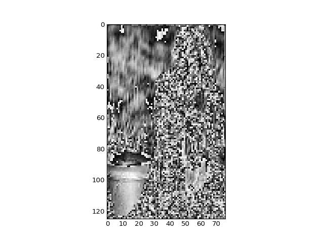
CNNs have multiple moving parts which can cause issues during training resulting in poor accuracy. Debugging problems in a CNN often start with investigating how the filters (kernels) are changing every iteration. Each weight used in a filter is constantly changing as the network attempts to learn the most accurate set of weights to use based on the train method.
In a well designed CNN, when the first convolution layer is started, the initialized input weights are set to be random (in this case using weight_init=tf.random_normal). These weights activate over an image and the output of the activation (feature map) is random as well. Visualizing the feature map as if it were an image, the output looks like the original image with static applied. The static is caused by all the weights activating at random. Over many iterations, each filter becomes more uniform as the weights are adjusted to fit the training feedback. As the network converges, the filters resemble distinct small patterns which can be found in the image.
Debugging a CNN requires a familiarity working with these filters. Currently there isn’t any built in support in tensorboard to display filters or feature maps. A simple view of the filters can be done using a tf.image_summary operation on the filters being trained and the feature maps generated. Adding an image summary output to a graph gives a good overview of the filters being used and the feature map generated by applying them to the input images.
An in progress jupyter notebook extension worth mentioning is TensorDebugger which is in an early state of development. The extension has a mode capable of viewing changes in filters as an animated gif over iterations.
# setup-only-ignore
filename_queue.close(cancel_pending_enqueues=True)
coord.request_stop()
coord.join(threads)
参考