CNN层
参考这里.
Common Layers
For a neural network architecture to be considered a CNN, it requires at least one convolution layer (tf.nn.conv2d). There are practical uses for a single layer CNN (edge detection), for image recognition and categorization it is common to use different layer types to support a convolution layer. These layers help reduce over-fitting, speed up training and decrease memory usage.
The layers covered in this chapter are focused on layers commonly used in a CNN architecture. A CNN isn’t limited to use only these layers, they can be mixed with layers designed for other network architectures.
# setup-only-ignore
import tensorflow as tf
import numpy as np
# setup-only-ignore
sess = tf.InteractiveSession()
Convolution Layers
One type of convolution layer has been covered in detail (tf.nn.conv2d) but there are a few notes which are useful to advanced users. The convolution layers in TensorFlow don’t do a full convolution, details can be found in the TensorFlow API documentation. In practice, the difference between a convolution and the operation TensorFlow uses is performance. TensorFlow uses a technique to speed up the convolution operation in all the different types of convolution layers.
There are use cases for each type of convolution layer but for tf.nn.conv2d is a good place to start. The other types of convolutions are useful but not required in building a network capable of object recognition and classification. A brief summary of each is included.
tf.nn.depthwise_conv2d
Used when attaching the output of one convolution to the input of another convolution layer. An advanced use case is using a tf.nn.depthwise_conv2d to create a network following the inception architecture.
tf.nn.separable_conv2d
Similar to tf.nn.conv2d but not a replacement. For large models, it speeds up training without sacrificing accuracy. For small models, it will converge quickly with worse accuracy.
tf.nn.conv2d_transpose
Applies a kernel to a new feature map where each section is filled with the same values as the kernel. As the kernel strides over the new image, any overlapping sections are summed together. There is a great explanation on how tf.nn.conv2d_transpose is used for learnable upsampling in Stanford’s CS231n Winter 2016: Lecture 13.
Activation Functions
These functions are used in combination with the output of other layers to generate a feature map. They’re used to smooth (or differentiate) the results of certain operations. The goal is to introduce non-linearity into the neural network. Non-linearity means that the input is a curve instead of a straight line. Curves are capable of representing more complex changes in input. For example, non-linear input is capable of describing input which stays small for the majority of the time but periodically has a single point at an extreme. Introduction of non-linearity in a neural network allows it to train on the complex patterns found in data.
TensorFlow has multiple activation functions available. With CNNs, tf.nn.relu is primarily used because of its performance although it sacrifices information. When starting out, using tf.nn.relu is recommended but advanced users may create their own. When considering if an activation function is useful there are a few primary considerations.
- The function is monotonic, so its output should always be increasing or decreasing along with the input. This allows gradient descent optimization to search for local minima.
- The function is differentiable, so there must be a derivative at any point in the function’s domain. This allows gradient descent optimization to properly work using the output from this style of activation function.
Any functions which satisfy those considerations could be used as activation functions. In TensorFlow there are a few worth highlighting which are common to see in CNN architectures. A brief summary of each is included with a small sample code illustrating their usage.
tf.nn.relu
A rectifier (rectified linear unit) called a ramp function in some documentation and looks like a skateboard ramp when plotted. ReLU is linear and keeps the same input values for any positive numbers while setting all negative numbers to be 0. It has the benefits that it doesn’t suffer from gradient vanishing and has a range of \([0,+\infty)\). A drawback of ReLU is that it can suffer from neurons becoming saturated when too high of a learning rate is used.
features = tf.range(-2, 3)
# Keep note of the value for negative features
sess.run([features, tf.nn.relu(features)])
[array([-2, -1, 0, 1, 2], dtype=int32), array([0, 0, 0, 1, 2], dtype=int32)]
In this example, the input in a rank one tensor (vector) of integer values between \([-2, 3]\). A tf.nn.relu is ran over the values the output highlights that any value less than 0 is set to be 0. The other input values are left untouched.
tf.sigmoid
A sigmoid function returns a value in the range of \([0.0, 1.0]\). Larger values sent into a tf.sigmoid will trend closer to 1.0 while smaller values will trend towards 0.0. The ability for sigmoids to keep a values between \([0.0, 1.0]\) is useful in networks which train on probabilities which are in the range of \([0.0, 1.0]\). The reduced range of output values can cause trouble with input becoming saturated and changes in input becoming exaggerated.
# Note, tf.sigmoid (tf.nn.sigmoid) is currently limited to float values
features = tf.to_float(tf.range(-1, 3))
sess.run([features, tf.sigmoid(features)])
[array([-1.,  0.,  1.,  2.], dtype=float32),
 array([ 0.26894143,  0.5       ,  0.7310586 ,  0.88079703], dtype=float32)]
In this example, a range of integers is converted to be float values (1 becomes 1.0) and a sigmoid function is ran over the input features. The result highlights that when a value of 0.0 is passed through a sigmoid, the result is 0.5 which is the midpoint of the simoid’s domain. It’s useful to note that with 0.5 being the sigmoid’s midpoint, negative values can be used as input to a sigmoid.
tf.tanh
A hyperbolic tangent function (tanh) is a close relative to tf.sigmoid with some of the same benefits and drawbacks. The main difference between tf.sigmoid and tf.tanh is that tf.tanh has a range of \([-1.0, 1.0]\). The ability to output negative values may be useful in certain network architectures.
# Note, tf.tanh (tf.nn.tanh) is currently limited to float values
features = tf.to_float(tf.range(-1, 3))
sess.run([features, tf.tanh(features)])
[array([-1.,  0.,  1.,  2.], dtype=float32),
 array([-0.76159418,  0.        ,  0.76159418,  0.96402758], dtype=float32)]
In this example, all the setup is the same as the tf.sigmoid example but the output shows an important difference. In the output of tf.tanh the midpoint is 0.0 with negative values. This can cause trouble if the next layer in the network isn’t expecting negative input or input of 0.0.
tf.nn.dropout
Set the output to be 0.0 based on a configurable probability. This layer performs well in scenarios where a little randomness helps training. An example scenario is when there are patterns being learned which are too tied to their neighboring features. This layer will add a little noise to the output being learned.
NOTE: This layer should only be used during training because the random noise it adds will give misleading results while testing.
features = tf.constant([-0.1, 0.0, 0.1, 0.2])
# Note, the output should be different on almost ever execution. Your numbers won't match
# this output.
sess.run([features, tf.nn.dropout(features, keep_prob=0.5)])
[array([-0.1,  0. ,  0.1,  0.2], dtype=float32),
 array([-0.        ,  0.        ,  0.        ,  0.40000001], dtype=float32)]
In this example, the output has a 50% probability of being kept. Each execution of this layer will have different output (most likely, it’s somewhat random). When an output is dropped, its value is set to 0.0.
Pooling Layers
Pooling layers reduce over-fitting and improving performance by reducing the size of the input. They’re used to scale down input while keeping important information for the next layer. It’s possible to reduce the size of the input using a tf.nn.conv2d alone but these layers execute much faster.
tf.nn.max_pool
Strides over a tensor and chooses the maximum value found within a certain kernel size. Useful when the intensity of the input data is relevant to importance in the image.
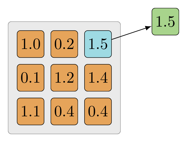
The same example is modeled using example code below. The goal is to find the largest value within the tensor.
# Usually the input would be output from a previous layer and not an image directly.
batch_size=1
input_height = 3
input_width = 3
input_channels = 1

layer_input = tf.constant([
        [
            [[1.0], [0.2], [1.5]],
            [[0.1], [1.2], [1.4]],
            [[1.1], [0.4], [0.4]]
        ]
    ])

# The strides will look at the entire input by using the image_height and image_width
kernel = [batch_size, input_height, input_width, input_channels]
max_pool = tf.nn.max_pool(layer_input, kernel, [1, 1, 1, 1], "VALID")
sess.run(max_pool)
array([[[[ 1.5]]]], dtype=float32)
The layer_input is a tensor with a shape similar to the output of tf.nn.conv2d or an activation function. The goal is to keep only one value, the largest value in the tensor. In this case, the largest value of the tensor is 1.5 and is returned in the same format as the input. If the kernel were set to be smaller, it would choose the largest value in each kernel size as it strides over the image.
Max-pooling will commonly be done using 2x2 receptive field (kernel with a height of 2 and width of 2) which is often written as a “2x2 max-pooling operation”. One reason to use a 2x2 receptive field is that it’s the smallest amount of downsampling which can be done in a single pass. If a 1x1 receptive field were used then the output would be the same as the input.
tf.nn.avg_pool
Strides over a tensor and averages all the values at each depth found within a kernel size. Useful when reducing values where the entire kernel is important, for example, input tensors with a large width and height but small depth.
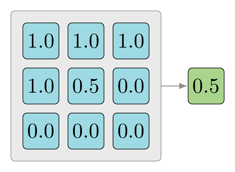
The same example is modeled using example code below. The goal is to find the average of all the values within the tensor.
batch_size=1
input_height = 3
input_width = 3
input_channels = 1

layer_input = tf.constant([
        [
            [[1.0], [1.0], [1.0]],
            [[1.0], [0.5], [0.0]],
            [[0.0], [0.0], [0.0]]
        ]
    ])

# The strides will look at the entire input by using the image_height and image_width
kernel = [batch_size, input_height, input_width, input_channels]
max_pool = tf.nn.avg_pool(layer_input, kernel, [1, 1, 1, 1], "VALID")
sess.run(max_pool)
array([[[[ 0.5]]]], dtype=float32)
Doing a summation of all the values in the tensor, then divide them by the size of the number of scalars in the tensor:
$$\dfrac{1.0 + 1.0 + 1.0 + 1.0 + 0.5 + 0.0 + 0.0 + 0.0 + 0.0}{9.0}$$
This is exactly what the example code did above but by reducing the size of the kernel, it’s possible to adjust the size of the output.
Normalization
Normalization layers are not unique to CNNs and aren’t used as often. When using tf.nn.relu, it is useful to consider normalization of the output. Since ReLU is unbounded, it’s often useful to utilize some form of normalization to identify high-frequency features.
tf.nn.local_response_normalization (tf.nn.lrn)
Local response normalization is a function which shapes the output based on a summation operation best explained in TensorFlow’s documentation.
… Within a given vector, each component is divided by the weighted, squared sum of inputs within depth_radius.
One goal of normalization is to keep the input in a range of acceptable numbers. For instance, normalizing input in the range of \([0.0,1.0]\) where the full range of possible values is normalized to be represented by a number greater than or equal to 0.0 and less than or equal to 1.0. Local response normalization normalizes values while taking into account the significance of each value.
Cuda-Convnet includes further details on why using local response normalization is useful in some CNN architectures. ImageNet uses this layer to normalize the output from tf.nn.relu.
# Create a range of 3 floats.
#  TensorShape([batch, image_height, image_width, image_channels])
layer_input = tf.constant([
        [[[ 1.]], [[ 2.]], [[ 3.]]]
    ])

lrn = tf.nn.local_response_normalization(layer_input)
sess.run([layer_input, lrn])
[array([[[[ 1.]],

         [[ 2.]],

         [[ 3.]]]], dtype=float32), array([[[[ 0.70710677]],

         [[ 0.89442718]],

         [[ 0.94868326]]]], dtype=float32)]
In this example code, the layer input is in the format [batch, image_height, image_width, image_channels]. The normalization reduced the output to be in the range of \([-1.0, 1.0]\). For tf.nn.relu, this layer will reduce its unbounded output to be in the same range.
High Level Layers
TensorFlow has introduced high level layers designed to make it easier to create fairly standard layer definitions. These aren’t required to use but they help avoid duplicate code while following best practices. While getting started, these layers add a number of non-essential nodes to the graph. It’s worth waiting until the basics are comfortable before using these layers.
tf.contrib.layers.convolution2d
The convolution2d layer will do the same logic as tf.nn.conv2d while including weight initialization, bias initialization, trainable variable output, bias addition and adding an activation function. Many of these steps haven’t been covered for CNNs yet but should be familiar. A kernel is a trainable variable (the CNN’s goal is to train this variable), weight initialization is used to fill the kernel with values (tf.truncated_normal) on its first run. The rest of the parameters are similar to what have been used before except they are reduced to short-hand version. Instead of declaring the full kernel, now it’s a simple tuple (1,1) for the kernel’s height and width.
image_input = tf.constant([
            [
                [[0., 0., 0.], [255., 255., 255.], [254., 0., 0.]],
                [[0., 191., 0.], [3., 108., 233.], [0., 191., 0.]],
                [[254., 0., 0.], [255., 255., 255.], [0., 0., 0.]]
            ]
        ])

conv2d = tf.contrib.layers.convolution2d(
    image_input,
    num_output_channels=4,
    kernel_size=(1,1),          # It's only the filter height and width.
    activation_fn=tf.nn.relu,
    stride=(1, 1),              # Skips the stride values for image_batch and input_channels.
    trainable=True)

# It's required to initialize the variables used in convolution2d's setup.
sess.run(tf.initialize_all_variables())
sess.run(conv2d)
array([[[[   0.        ,    0.        ,    0.        ,    0.        ],
         [ 166.44549561,    0.        ,    0.        ,    0.        ],
         [ 171.00466919,    0.        ,    0.        ,    0.        ]],

        [[  28.54177475,    0.        ,   59.9046936 ,    0.        ],
         [   0.        ,  124.69891357,    0.        ,    0.        ],
         [  28.54177475,    0.        ,   59.9046936 ,    0.        ]],

        [[ 171.00466919,    0.        ,    0.        ,    0.        ],
         [ 166.44549561,    0.        ,    0.        ,    0.        ],
         [   0.        ,    0.        ,    0.        ,    0.        ]]]], dtype=float32)
This example setup a full convolution against a batch of a single image. All the parameters are based off of the steps done throughout this chapter. The main difference is that tf.contrib.layers.convolution2d does a large amount of setup without having to write it all again. This can be a great time saving layer for advanced users.
NOTE: tf.to_float should not be used if the input is an image, instead use tf.image.convert_image_dtype which will properly change the range of values used to describe colors. In this example code, float values of 255. were used which aren’t what TensorFlow expects when is sees an image using float values. TensorFlow expects an image with colors described as floats to stay in the range of \([0,1]\).
tf.contrib.layers.fully_connected
A fully connected layer is one where every input is connected to every output. This is a fairly common layer in many architectures but for CNNs, the last layer is quite often fully connected. The tf.contrib.layers.fully_connected layer offers a great short-hand to create this last layer while following best practices.
Typical fully connected layers in TensorFlow are often in the format of tf.matmul(features, weight) + bias where feature, weight and bias are all tensors. This short-hand layer will do the same thing while taking care of the intricacies involved in managing the weight and bias tensors.
features = tf.constant([
        [[1.2], [3.4]]
    ])

fc = tf.contrib.layers.fully_connected(features, num_output_units=2)
# It's required to initialize all the variables first or there'll be an error about precondition failures.
sess.run(tf.initialize_all_variables())
sess.run(fc)
array([[[-0.53210509,  0.74457598],
        [-1.50763106,  2.10963178]]], dtype=float32)
This example created a fully connected layer and associated the input tensor with each neuron of the output. There are plenty of other parameters to tweak for different fully connected layers.
Layer Input
Each layer serves a purpose in a CNN architecture. It’s important to understand them at a high level (at least) but without practice they’re easy to forget. A crucial layer in any neural network is the input layer, where raw input is sent to be trained and tested. For object recognition and classification, the input layer is a tf.nn.conv2d layer which accepts images. The next step is to use real images in training instead of example input in the form of tf.constant or tf.range variables.