线性回归
线性回归是最简单的回归方法,它的目标是使用超平面拟合数据集,即学习一个线性模型以尽可能准确的预测实值输出标记。
单变量模型
模型
$$f(x)=w^Tx+b$$
在线性回归问题中,一般使用最小二乘参数估计($$L_2$$损失),定义目标函数为
$$J={\arg min}{(w,b)}\sum{i=1}^{m}(y_i-wx_i-b)^2$$
均方误差(MSE)
$$MSE = \frac{1}{N} \sum_{i=1}^{m}{(y_i-wx_i-b)^2}$$
多变量模型
多变量时可以表示为矩阵
$$f(X)=W^TX+b=\hat{W}X’$$ $$\hat{W}=(W, b), X’=(X, 1)$$
目标函数为
$$J={\arg min}_{W}(y-X\hat{W})^T(y-X\hat{W})$$
当 $X^TX$ 为满秩矩阵时,可以得到最优解
$$\hat{W}=(X^TX)^{-1}X^Ty$$
注意:
- 多变量时需要对输入数据作归一化,如 $$x=\frac{x-u}{x_{max}-x_{min}}$$
- 实际计算过程中(如使用梯度下降算法)学习率的选择方法
- 收敛慢时,增大学习率
- 不收敛时,减小学习率
- 学习率的选择规则一般为
..., 0.001, 0.01, 0.1, 1, 10, ...
示例
生成数据
#Indicate the matplotlib to show the graphics inline
%matplotlib inline
import matplotlib.pyplot as plt # import matplotlib
import numpy as np # import numpy
import tensorflow as tf
import numpy as np
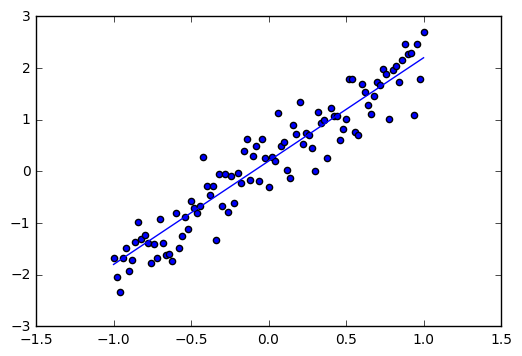
trX = np.linspace(-1, 1, 101) #Create a linear space of 101 points between 1 and 1
trY = 2 * trX + np.random.randn(*trX.shape) * 0.4 + 0.2 #Create The y function based on the x axis
plt.figure() # Create a new figure
plt.scatter(trX,trY) #Plot a scatter draw of the random datapoints
plt.plot (trX, .2 + 2 * trX) # Draw one line with the line function
单变量示例
#!/usr/bin/env python
# h(X)= b + wX
%matplotlib inline
import tensorflow as tf
import numpy as np
import matplotlib.pyplot as plt
def model(X, w, b):
return tf.mul(X, w) + b
trX = np.linspace(-1, 1, 101).astype(np.float32)
# create a y value which is approximately linear but with some random noise
trY = 2 * trX + np.random.randn(*trX.shape) * 0.33 + 10
# create a shared variable (like theano.shared) for the weight matrix
w = tf.Variable(tf.random_uniform([1], -1.0, 1.0))
b = tf.Variable(tf.zeros([1]))
cost = tf.reduce_mean(tf.square(trY-model(trX, w, b)))
# construct an optimizer to minimize cost and fit line to my data
train_op = tf.train.GradientDescentOptimizer(0.01).minimize(cost)
# Launch the graph in a session
with tf.Session() as sess:
# you need to initialize variables (in this case just variable W)
tf.initialize_all_variables().run()
for i in range(1000):
sess.run(train_op)
print "w should be something around [2]:", sess.run(w)
print "b should be something around [10]:", sess.run(b)
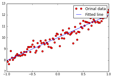
plt.plot(trX, trY, "ro", label="Orinal data")
plt.plot(trX, w.eval()*trX + b.eval(), label="Fitted line")
plt.legend()
plt.show()
# Plot with pandas
#import pandas as pd
#fig, axes = plt.subplots(nrows=1, ncols=1)
#pd.DataFrame({'x':trX,'y':trY}).plot.scatter(x='x', y='y', ax=axes, color='red')
#pd.DataFrame({'x':trX,'y':w.eval()*trX + b.eval()}).plot.scatter(x='x', y='y', ax=axes, color='blue')
w should be something around [2]:  [ 2.00981951]
b should be something around [10]: [ 9.98865509]
多变量示例
多变量其实就是输入变成了矩阵:
#!/usr/bin/env python
# h(X)= B + WX
%matplotlib inline
import tensorflow as tf
import numpy as np
import matplotlib.pyplot as plt

def model(X, w, b):
    return tf.mul(w, X) + b

trX = np.mgrid[-1:1:0.01, -10:10:0.1].reshape(2, -1).T
trW = np.array([3, 5])
trY = trW*trX + np.random.randn(*trX.shape) + [20, 100]

w = tf.Variable(np.array([1., 1.]).astype(np.float32))
b = tf.Variable(np.array([[1., 1.]]).astype(np.float32))
cost = tf.reduce_mean(tf.square(trY-model(trX, w, b)))

# construct an optimizer to minimize cost and fit line to my data
train_op = tf.train.GradientDescentOptimizer(0.05).minimize(cost)

# Launch the graph in a session
with tf.Session() as sess:
    # you need to initialize variables (in this case just variable W)
    tf.initialize_all_variables().run()

    for i in range(1000):
        if i % 99 == 0:
            print "Cost at step", i, "is:", cost.eval()
        sess.run(train_op)

    print "w should be something around [3, 5]:", sess.run(w)
    print "b should be something around [20,100]:", sess.run(b)
Cost at step 0 is: 5329.87
Cost at step 99 is: 1.22204
Cost at step 198 is: 0.998043
Cost at step 297 is: 0.997083
Cost at step 396 is: 0.997049
Cost at step 495 is: 0.997049
Cost at step 594 is: 0.997049
Cost at step 693 is: 0.997049
Cost at step 792 is: 0.997049
Cost at step 891 is: 0.997049
Cost at step 990 is: 0.997049
w should be something around [3, 5]:  [ 3.00108743  5.00054932]
b should be something around [20,100]: [[  20.00317383  100.00382233]]
tensorflow 示例
import tensorflow as tf

# initialize variables/model parameters
W = tf.Variable(tf.zeros([2, 1]), name="weights")
b = tf.Variable(0., name="bias")

def inference(X):
    # compute inference model over data X and return the result
    return tf.matmul(X, W) + b

def loss(X, Y):
    # compute loss over training data X and expected outputs Y
    Y_predicted = inference(X)
    return tf.reduce_sum(tf.squared_difference(Y, Y_predicted))

def inputs():
    # read/generate input training data X and expected outputs Y
    weight_age = [[84, 46], [73, 20], [65, 52], [70, 30], [76, 57], [69, 25], [63, 28], [72, 36], [79, 57], [75, 44], [27, 24], [89, 31], [65, 52], [57, 23], [59, 60], [69, 48], [60, 34], [79, 51], [75, 50], [82, 34], [59, 46], [67, 23], [85, 37], [55, 40], [63, 30]]
    blood_fat_content = [354, 190, 405, 263, 451, 302, 288, 385, 402, 365, 209, 290, 346, 254, 395, 434, 220, 374, 308, 220, 311, 181, 274, 303, 244]

    return tf.to_float(weight_age), tf.to_float(blood_fat_content)

def train(total_loss):
    # train / adjust model parameters according to computed total loss
    learning_rate = 0.000001
    return tf.train.GradientDescentOptimizer(learning_rate).minimize(total_loss)


def evaluate(sess, X, Y):
    # evaluate the resulting trained model
    print sess.run(inference([[80., 25.]])) # ~ 303
    print sess.run(inference([[65., 25.]])) # ~ 256

# Create a saver.
# saver = tf.train.Saver()

# Launch the graph in a session, setup boilerplate
with tf.Session() as sess:
    tf.initialize_all_variables().run()

    X, Y = inputs()

    total_loss = loss(X, Y)
    train_op = train(total_loss)

    coord = tf.train.Coordinator()
    threads = tf.train.start_queue_runners(sess=sess, coord=coord)

    # actual training loop
    training_steps = 1000
    for step in range(training_steps):
        sess.run([train_op])
        # for debugging and learning purposes, see how the loss gets decremented
        # through training steps
        if step % 10 == 0:
            print "loss at step", step, ":", sess.run([total_loss])
        # save training checkpoints in case loosing them
        # if step % 1000 == 0:
        #     saver.save(sess, 'my-model', global_step=step)

    evaluate(sess, X, Y)
    coord.request_stop()
    coord.join(threads)
    # saver.save(sess, 'my-model', global_step=training_steps)
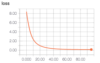
输出:
loss at step  0 : [54929292.0]
loss at step  10 : [14629748.0]
loss at step  20 : [7090800.0]
loss at step  30 : [5680201.0]
loss at step  40 : [5416011.0]
loss at step  50 : [5366280.5]
loss at step  60 : [5356678.0]
loss at step  70 : [5354588.0]
loss at step  80 : [5353913.0]
loss at step  90 : [5353510.0]
loss at step  100 : [5353166.0]
loss at step  110 : [5352839.5]
loss at step  120 : [5352525.0]
loss at step  130 : [5352218.5]
loss at step  140 : [5351921.0]
loss at step  150 : [5351631.5]
loss at step  160 : [5351349.0]
loss at step  170 : [5351075.0]
loss at step  180 : [5350808.0]
loss at step  190 : [5350549.5]
loss at step  200 : [5350297.0]
loss at step  210 : [5350050.5]
loss at step  220 : [5349814.0]
loss at step  230 : [5349580.5]
loss at step  240 : [5349356.0]
loss at step  250 : [5349134.0]
loss at step  260 : [5348922.0]
loss at step  270 : [5348712.5]
loss at step  280 : [5348511.5]
loss at step  290 : [5348313.5]
loss at step  300 : [5348123.5]
loss at step  310 : [5347935.0]
loss at step  320 : [5347753.5]
loss at step  330 : [5347577.5]
loss at step  340 : [5347405.0]
loss at step  350 : [5347237.0]
loss at step  360 : [5347073.0]
loss at step  370 : [5346915.0]
loss at step  380 : [5346761.0]
loss at step  390 : [5346611.0]
loss at step  400 : [5346464.5]
loss at step  410 : [5346320.5]
loss at step  420 : [5346182.5]
loss at step  430 : [5346047.5]
loss at step  440 : [5345914.0]
loss at step  450 : [5345786.0]
loss at step  460 : [5345662.0]
loss at step  470 : [5345539.5]
loss at step  480 : [5345420.5]
loss at step  490 : [5345305.5]
loss at step  500 : [5345193.0]
loss at step  510 : [5345082.5]
loss at step  520 : [5344976.5]
loss at step  530 : [5344871.0]
loss at step  540 : [5344771.0]
loss at step  550 : [5344670.5]
loss at step  560 : [5344574.5]
loss at step  570 : [5344480.5]
loss at step  580 : [5344388.0]
loss at step  590 : [5344298.0]
loss at step  600 : [5344212.0]
loss at step  610 : [5344127.0]
loss at step  620 : [5344042.5]
loss at step  630 : [5343962.0]
loss at step  640 : [5343882.0]
loss at step  650 : [5343805.5]
loss at step  660 : [5343729.5]
loss at step  670 : [5343657.0]
loss at step  680 : [5343584.0]
loss at step  690 : [5343514.5]
loss at step  700 : [5343446.5]
loss at step  710 : [5343380.0]
loss at step  720 : [5343314.5]
loss at step  730 : [5343250.0]
loss at step  740 : [5343187.5]
loss at step  750 : [5343128.0]
loss at step  760 : [5343067.5]
loss at step  770 : [5343010.5]
loss at step  780 : [5342952.5]
loss at step  790 : [5342897.5]
loss at step  800 : [5342843.0]
loss at step  810 : [5342791.5]
loss at step  820 : [5342738.5]
loss at step  830 : [5342688.5]
loss at step  840 : [5342638.5]
loss at step  850 : [5342589.5]
loss at step  860 : [5342543.0]
loss at step  870 : [5342496.5]
loss at step  880 : [5342449.5]
loss at step  890 : [5342406.0]
loss at step  900 : [5342363.0]
loss at step  910 : [5342319.5]
loss at step  920 : [5342277.5]
loss at step  930 : [5342236.0]
loss at step  940 : [5342197.5]
loss at step  950 : [5342157.0]
loss at step  960 : [5342118.5]
loss at step  970 : [5342080.5]
loss at step  980 : [5342043.0]
loss at step  990 : [5342007.5]
[[318.77984619]]
[[266.52853394]]
sklearn 示例
import tensorflow.contrib.learn.python.learn as learn
from sklearn import datasets, metrics, preprocessing

boston = datasets.load_boston()
x = preprocessing.StandardScaler().fit_transform(boston.data)
feature_columns = learn.infer_real_valued_columns_from_input(x)
regressor = learn.LinearRegressor(feature_columns=feature_columns)
regressor.fit(x, boston.target, steps=200, batch_size=32)
boston_predictions = list(regressor.predict(x, as_iterable=True))
score = metrics.mean_squared_error(boston_predictions, boston.target)
print ("MSE: %f" % score)